API (beta)
ccplot >= 1.5-rc5
If the command-line program does not fulfill your needs, you can use routines provided with ccplot to make custom plots in python. These include routines for reading HDF and HDF-EOS2 files, parsing time values and performing data interpolation. See API reference for details.
Examples
Note about examples
The examples below differ from the ccplot program in a number of important details:
-
The aspect ratio is determined by matplotlib. The figure size is fixed in inches, so the actual aspect ratio depends on the horizontal and vertical extent. In contrast, the ccplot program sets the figure width according to a prespecified aspect ratio.
-
A new interpolation routine ccplot.algorithms.interp2d_12 is used, which performs interpolation by averaging as opposed to nearest-neighbor interpolation in the ccplot program (but see API reference for details).
CALIPSO example
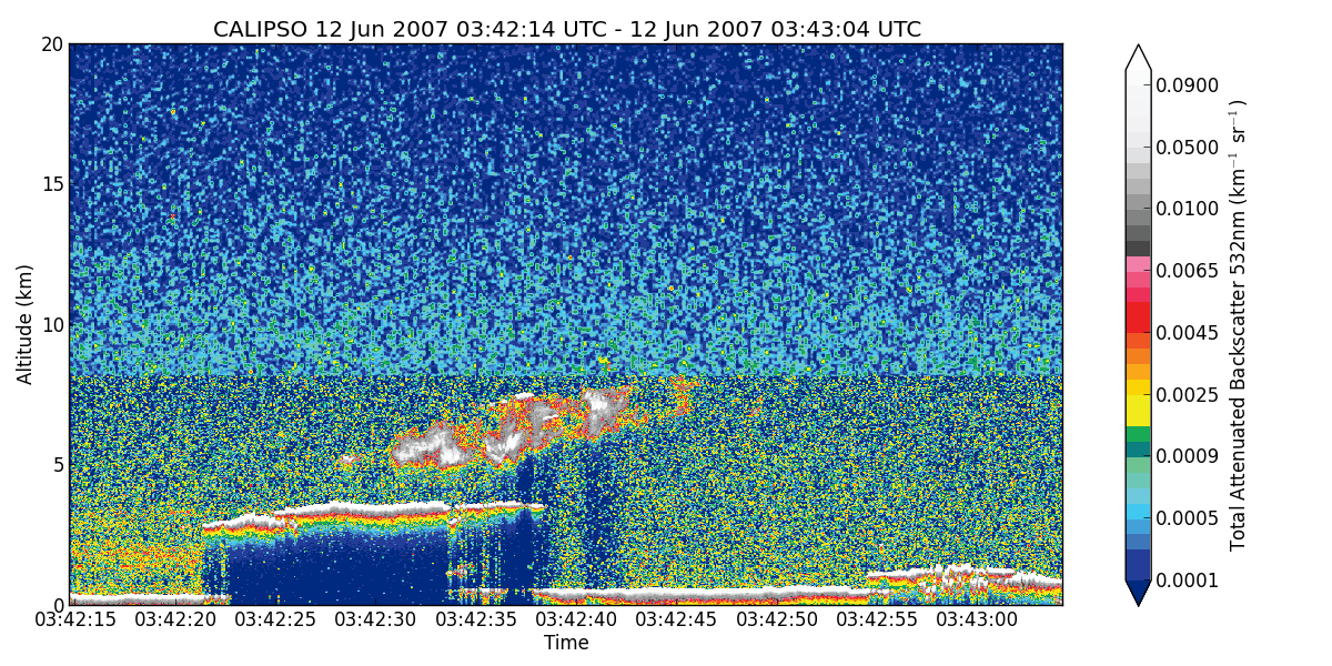
Input file: CAL_LID_L1-ValStage1-V3-01.2007-06-12T03-42-18ZN.hdf
Source: calipso-plot.py
#!/usr/bin/env python3

import os
import numpy as np
import matplotlib as mpl
import matplotlib.pyplot as plt
from ccplot.hdf import HDF
from ccplot.algorithms import interp2d_12
import ccplot.utils
import ccplot.config

filename = 'CAL_LID_L1-ValStage1-V3-01.2007-06-12T03-42-18ZN.hdf'
name = 'Total_Attenuated_Backscatter_532'
label = 'Total Attenuated Backscatter 532nm (km$^{-1}$ sr$^{-1}$)'
colormap = os.path.join(ccplot.config.sharepath, 'cmap', 'calipso-backscatter.cmap')
x1 = 0
x2 = 1000
h1 = 0  # km
h2 = 20  # km
nz = 500  # Number of pixels in the vertical.

if __name__ == '__main__':
    with HDF(filename) as product:
        # Import datasets.
        time = product['Profile_UTC_Time'][x1:x2, 0]
        height = product['metadata']['Lidar_Data_Altitudes']
        dataset = product[name][x1:x2]

        # Convert time to datetime.
        time = np.array([ccplot.utils.calipso_time2dt(t) for t in time])

        # Mask missing values.
        dataset = np.ma.masked_equal(dataset, -9999)

        # Interpolate data on a regular grid.
        X = np.arange(x1, x2, dtype=np.float32)
        Z, null = np.meshgrid(height, X)
        data = interp2d_12(
            dataset[::],
            X.astype(np.float32),
            Z.astype(np.float32),
            x1, x2, x2 - x1,
            h2, h1, nz,
        )

        # Import colormap.
        cmap = ccplot.utils.cmap(colormap)
        cm = mpl.colors.ListedColormap(cmap['colors']/255.0)
        cm.set_under(cmap['under']/255.0)
        cm.set_over(cmap['over']/255.0)
        cm.set_bad(cmap['bad']/255.0)
        norm = mpl.colors.BoundaryNorm(cmap['bounds'], cm.N)

        # Plot figure.
        fig = plt.figure(figsize=(12, 6))
        TIME_FORMAT = '%e %b %Y %H:%M:%S UTC'
        im = plt.imshow(
            data.T,
            extent=(mpl.dates.date2num(time[0]), mpl.dates.date2num(time[-1]), h1, h2),
            cmap=cm,
            norm=norm,
            aspect='auto',
            interpolation='nearest',
        )
        ax = im.axes
        ax.set_title('CALIPSO %s - %s' % (
            time[0].strftime(TIME_FORMAT),
            time[-1].strftime(TIME_FORMAT)
        ))
        ax.set_xlabel('Time')
        ax.set_ylabel('Altitude (km)')
        ax.xaxis.set_major_locator(mpl.dates.AutoDateLocator())
        ax.xaxis.set_major_formatter(mpl.dates.DateFormatter('%H:%M:%S'))
        cbar = plt.colorbar(
            extend='both',
            use_gridspec=True
        )
        cbar.set_label(label)
        fig.tight_layout()
        plt.savefig('calipso-plot.png')
        plt.show()
CloudSat example
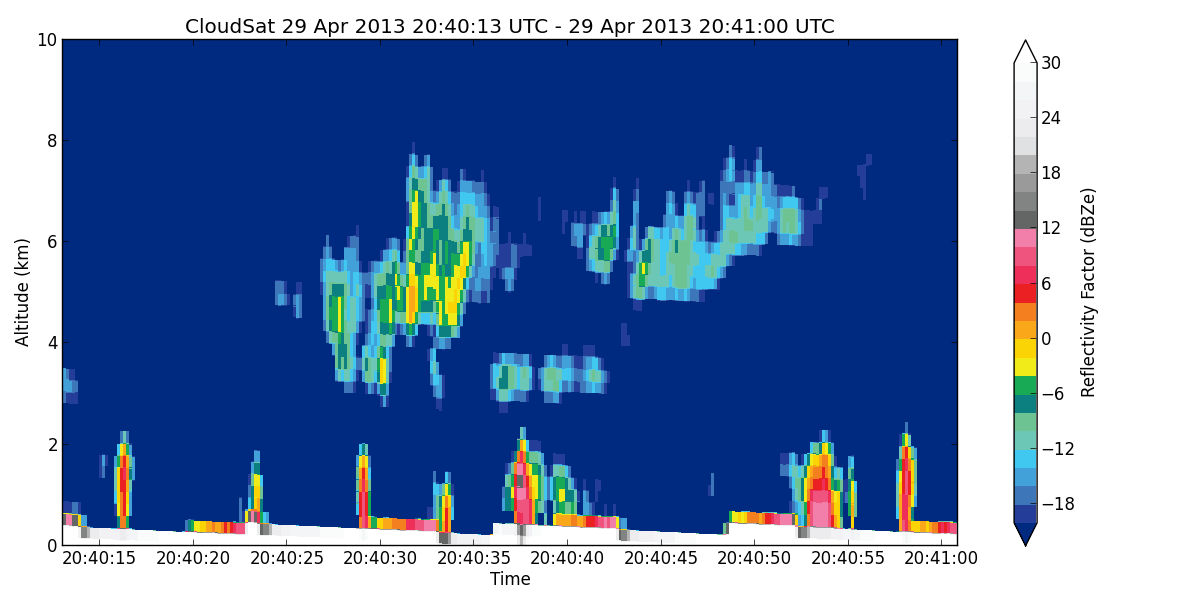
Input file: 2013119200420_37263_CS_2B-GEOPROF_GRANULE_P_R04_E06.hdf
Source: cloudsat-plot.py
#!/usr/bin/env python3

import os
import numpy as np
import matplotlib as mpl
import matplotlib.pyplot as plt
import datetime as dt
from ccplot.hdfeos import HDFEOS
from ccplot.algorithms import interp2d_12
import ccplot.utils
import ccplot.config

filename = '2013119200420_37263_CS_2B-GEOPROF_GRANULE_P_R04_E06.hdf'
swath = '2B-GEOPROF'
name = 'Radar_Reflectivity'
label = 'Reflectivity Factor (dBZe)'
colormap = os.path.join(ccplot.config.sharepath, 'cmap', 'cloudsat-reflectivity.cmap')
x1 = 1700
x2 = 2000
h1 = 0  # km
h2 = 10  # km
nz = 500  # Number of pixels in the vertical.

if __name__ == '__main__':
    with HDFEOS(filename) as product:
        # Import datasets.
        sw = product[swath]
        ds = sw[name]
        dataset = ds[x1:x2]
        time = sw['Profile_time'][x1:x2]
        height = sw['Height'][:]
        start_time = dt.datetime.strptime(
            sw.attributes['start_time'],
            '%Y%m%d%H%M%S'
        )

        # Convert time to datetime.
        time = np.array([
            ccplot.utils.cloudsat_time2dt(t, start_time)
            for t in time
        ])

        # Mask missing values.
        dataset = np.ma.masked_equal(dataset, ds.attributes['missing'])
        dataset = np.ma.masked_equal(dataset, ds.attributes['_FillValue'])

        # Transform data values to science values.
        factor = ds.attributes.get('factor', 1)
        offset = ds.attributes.get('offset', 0)
        dataset = 1.0/factor*(dataset - offset)

        # Interpolate data on a regular grid.
        X = np.arange(x1, x2, dtype=np.float32)
        Z = (height*0.001).astype(np.float32)
        data = interp2d_12(
            dataset.filled(np.nan), X, Z,
            x1, x2, x2 - x1,
            h2, h1, nz,
        )

        # Import colormap.
        cmap = ccplot.utils.cmap(colormap)
        cm = mpl.colors.ListedColormap(cmap['colors']/255.0)
        cm.set_under(cmap['under']/255.0)
        cm.set_over(cmap['over']/255.0)
        cm.set_bad(cmap['bad']/255.0)
        norm = mpl.colors.BoundaryNorm(cmap['bounds'], cm.N)

        # Plot figure.
        fig = plt.figure(figsize=(12, 6))
        TIME_FORMAT = '%e %b %Y %H:%M:%S UTC'
        im = plt.imshow(
            data.T,
            extent=(mpl.dates.date2num(time[0]), mpl.dates.date2num(time[-1]), h1, h2),
            cmap=cm,
            norm=norm,
            aspect='auto',
            interpolation='nearest',
        )
        ax = im.axes
        ax.set_title('CloudSat %s - %s' % (
            time[0].strftime(TIME_FORMAT),
            time[-1].strftime(TIME_FORMAT)
        ))
        ax.set_xlabel('Time')
        ax.set_ylabel('Altitude (km)')
        ax.xaxis.set_major_locator(mpl.dates.AutoDateLocator())
        ax.xaxis.set_major_formatter(mpl.dates.DateFormatter('%H:%M:%S'))
        cbar = plt.colorbar(
            extend='both',
            use_gridspec=True
        )
        cbar.set_label(label)
        fig.tight_layout()
        plt.savefig('cloudsat-plot.png')
        plt.show()